在之前的课程中我们学习了如何使用 Stata 绘制粤港澳大湾区的地图:如何使用 Stata 绘制粤港澳大湾区的地图? 。 最近有个小伙伴询问关于这幅地图的绘制方法:
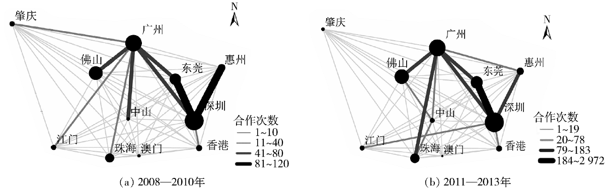
参考图
群里的其他小伙伴提出了很多方法,有说用 MATLAB 的,有说用 Gephi 的。实际上这幅图用 Stata 就可以画出来!
需要注意上面的图中,各个城市的相对位置实际上就是其空间相对位置,我怀疑作者可能是为了避免审图的麻烦而把地图底图删去了,完整的地图可能是这样的:
完整地图
我们今天就一起学习下如何使用 Stata 绘制空间网络图。
详细的内容可以参加明晚的课程学习,下面介绍下大致的方法。
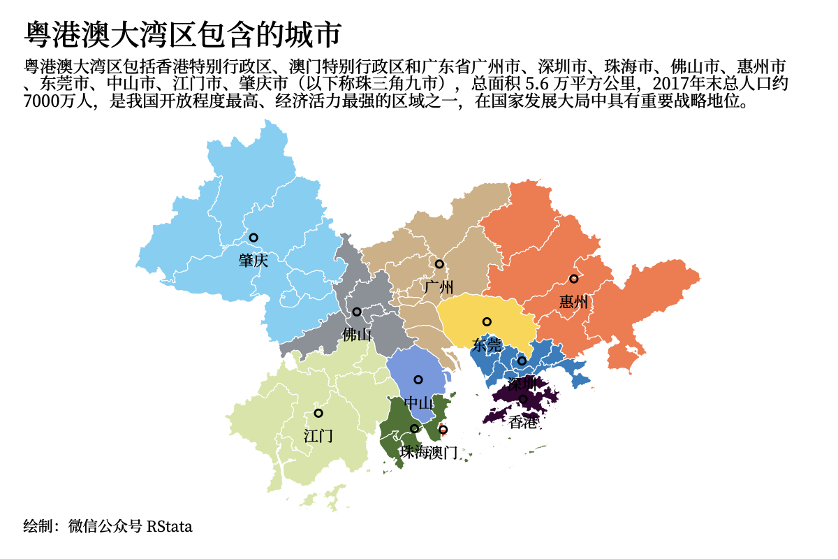
首先我们可以使用 spmap 绘制一幅大湾区的地图:
use yga_county_db2.dta, clear encode 市, gen (city)tab city if wq, nolabelspmap city using yga_county_coord.dta if wq, id(ID) clmethod(custom) clbreaks(0 1 2 4 5 6 11 13 17 18 19 23) fcolor("254 212 57" "112 154 225" "138 145 151" "210 175 129" "253 116 70" "213 228 162" "25 126 192" "240 92 59" "70 115 46" "113 208 245" "55 3 53" ) leg(off) ocolor("white" ...) osize(vthin ...) point(data(yga_db2.dta) x(x) y (y) size(*0.5 ...) osize(*1.2 ...) select(keep if wq) shape(Oh)) label (data(yga_db2.dta) x(x) y (y) label (市) gap(*1.8) pos(6) length (6) select(keep if wq)) graphr(margin(medium)) xsize(9) ysize(6) ti("粤港澳大湾区包含的城市" , size(*1.1) pos(11)) subti("粤港澳大湾区包括香港特别行政区、澳门特别行政区和广东省广州市、深圳市、珠海市、佛山市、惠州市" "、东莞市、中山市、江门市、肇庆市(以下称珠三角九市),总面积 5.6 万平方公里,2017年末总人口约" "7000万人,是我国开放程度最高、经济活力最强的区域之一,在国家发展大局中具有重要战略地位。" , size(*0.8) pos(11)) caption("绘制:微信公众号 RStata" , size(*0.8))
大湾区地图
然后使用 arrow() 选项即可在地图上添加空间网络图,不过在此之前我们需要先构造 arrow() 的数据,根据帮助文档的介绍,arrow() 数据需要类似这样:
* An arrow dataset is a Stata dataset that contains the definition of one
* or more arrows to be superimposed onto the base map. An arrow dataset is
* required to have the following structure:

*          _ID       _X1       _Y1       _X2       _Y2   byvar_ar
*        ---------------------------------------------------------
*            1        11        30        18        30          1
*            2        15        40        15        45          1
*            3        15        40        25        40          1
*            4        20        35        28        45          2
*            5        17        20        20        11          2
*        ---------------------------------------------------------

* _ID is required and is a numeric variable that uniquely identifies the
* arrows. _X1 is required and is a numeric variable that contains the
* x-coordinate of the starting point of the arrows. _Y1 is required and is
* a numeric variable that contains the y-coordinate of the starting point
* of the arrows. _X2 is required and is a numeric variable that contains
* the x-coordinate of the ending point of the arrows. _Y2 is required and
* is a numeric variable that contains the y-coordinate of the ending point
* of the arrows. Finally, byvar_ar is a placeholder denoting an optional
* variable that can be specified to distinguish different kinds of arrows.
也就是要包含 _ID, _X1, _X2, _Y1, _Y2 五个变量,还有一个分组变量。
我准备了一个示例数据:
use yga_db.dta, clear ren ID _IDmerge 1:m _ID using yga_coord.dtakeep 市 *_centroidduplicates drop _all, forcegen to = substr (市, 1, 6)ren 市 fromsave centroid, replace import excel using "示例数据.xlsx" , clear first merge m :1 from using centroidkeep if _m == 3drop _mren x_centroid _X1ren y_centroid _Y1merge m :1 to using centroidkeep if _m == 3drop _mren x_centroid _X2ren y_centroid _Y2bysort year: gen _ID = _nhist value if substr (from, 1, 6) != torecode value (0/25 = 1) (26/50 = 2) (51/75 = 3) (76/. = 4), gen (group)tab groupgsort groupsave arrow, replace
另外我们还需要使用散点的大小表示总 value 的量:
use arrow, clear collapse (sum ) sum = value, by (to)ren to 市save sum , replace use yga_db2.dta, clear replace 市 = substr (市, 1, 6)merge 1:1 市 using sum keep if wqdrop group _mhist sum recode sum (0/800 = 1) (801/900 = 2) (901/1000 = 3) (1001/. = 4), gen (group)tab groupsave label , replace
然后就可以绘制地图了:
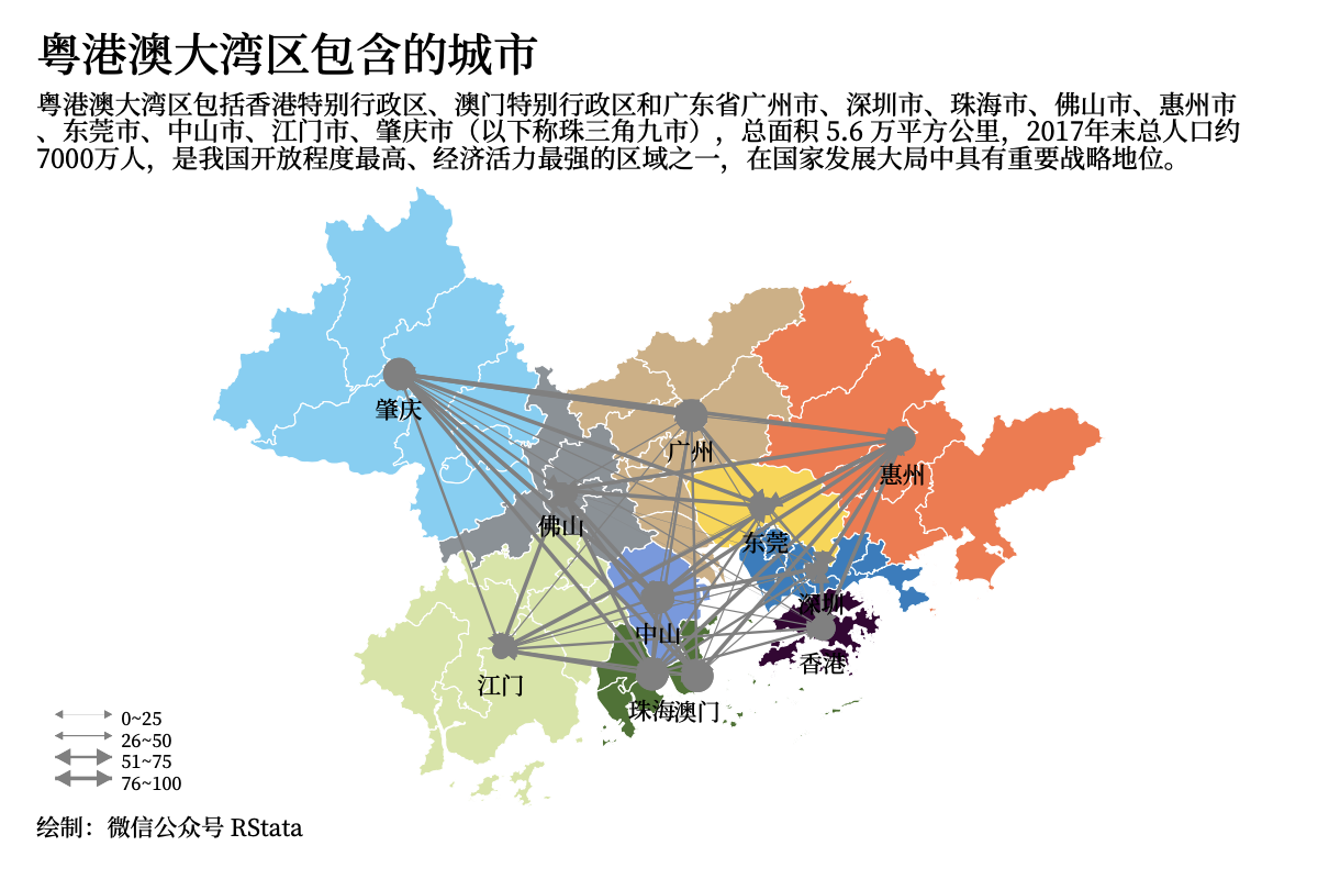
use yga_county_db2.dta, clear encode 市, gen (city)tab city if wq, nolabelspmap city using yga_county_coord.dta if wq, id(ID) clmethod(custom) clbreaks(0 1 2 4 5 6 11 13 17 18 19 23) fcolor("254 212 57" "112 154 225" "138 145 151" "210 175 129" "253 116 70" "213 228 162" "25 126 192" "240 92 59" "70 115 46" "113 208 245" "55 3 53" ) ocolor("white" ...) osize(vthin ...) point(data(label ) x(x) y (y) by (group) size(*0.5 *1 *1.5 *2) osize(*1.2 ...) shape(O) fcolor(gray ...) ocolor(gray ...)) label (data(label ) x(x) y (y) label (市) gap(*1.8) pos(6) length (6)) graphr(margin(medium)) xsize(9) ysize(6) ti("粤港澳大湾区包含的城市" , size(*1.1) pos(11)) subti("粤港澳大湾区包括香港特别行政区、澳门特别行政区和广东省广州市、深圳市、珠海市、佛山市、惠州市" "、东莞市、中山市、江门市、肇庆市(以下称珠三角九市),总面积 5.6 万平方公里,2017年末总人口约" "7000万人,是我国开放程度最高、经济活力最强的区域之一,在国家发展大局中具有重要战略地位。" , size(*0.8) pos(11)) caption("绘制:微信公众号 RStata" , size(*0.8)) arrow(data(arrow) by (group) select(keep if year == 2020) direction(2 ...) legenda(on ) legcount lsize(*0.1 *0.5 *1 *1.5) lcolor(gray ...) hfcolor(gray ...) hocolor(gray ...) hsize(1 1 2 2) hbarbsize(1 1 2 2)) leg(order (17 "0~25" 18 "26~50" 19 "51~75" 20 "76~100" ) symxsize(*2)) gr export "粤港澳湾区城市空间网络关系图.png" , replace width(1200)
粤港澳湾区城市空间网络关系图
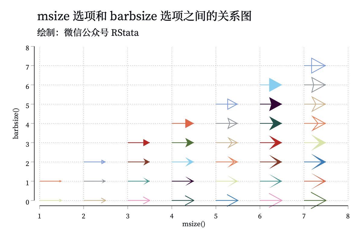
关于箭头的设置有两个选项,msize() 和 barbsize(),这两个选项的不同组合会绘制出不同形状的箭头:
msize() 和 barbsize()
local cmd
forval x = 1/7{
	forval y = 0/`x'{
		local x1 = `x' + 0.5
		local cmd (pcarrowi `y' `x' `y' `x1', msize(`x') barbsize(`y')) `cmd'
	}
}

di `"`cmd'"'
tw `cmd', yla(0(1)8, ang(0)) xla(1(1)8) leg(off) ///
	yti("barbsize()") xti("msize()") ///
	plotr(color(white)) ///
	ti("msize 选项和 barbsize 选项之间的关系图") ///
	sch(lightrstata) ///
	subti("绘制:微信公众号 RStata")
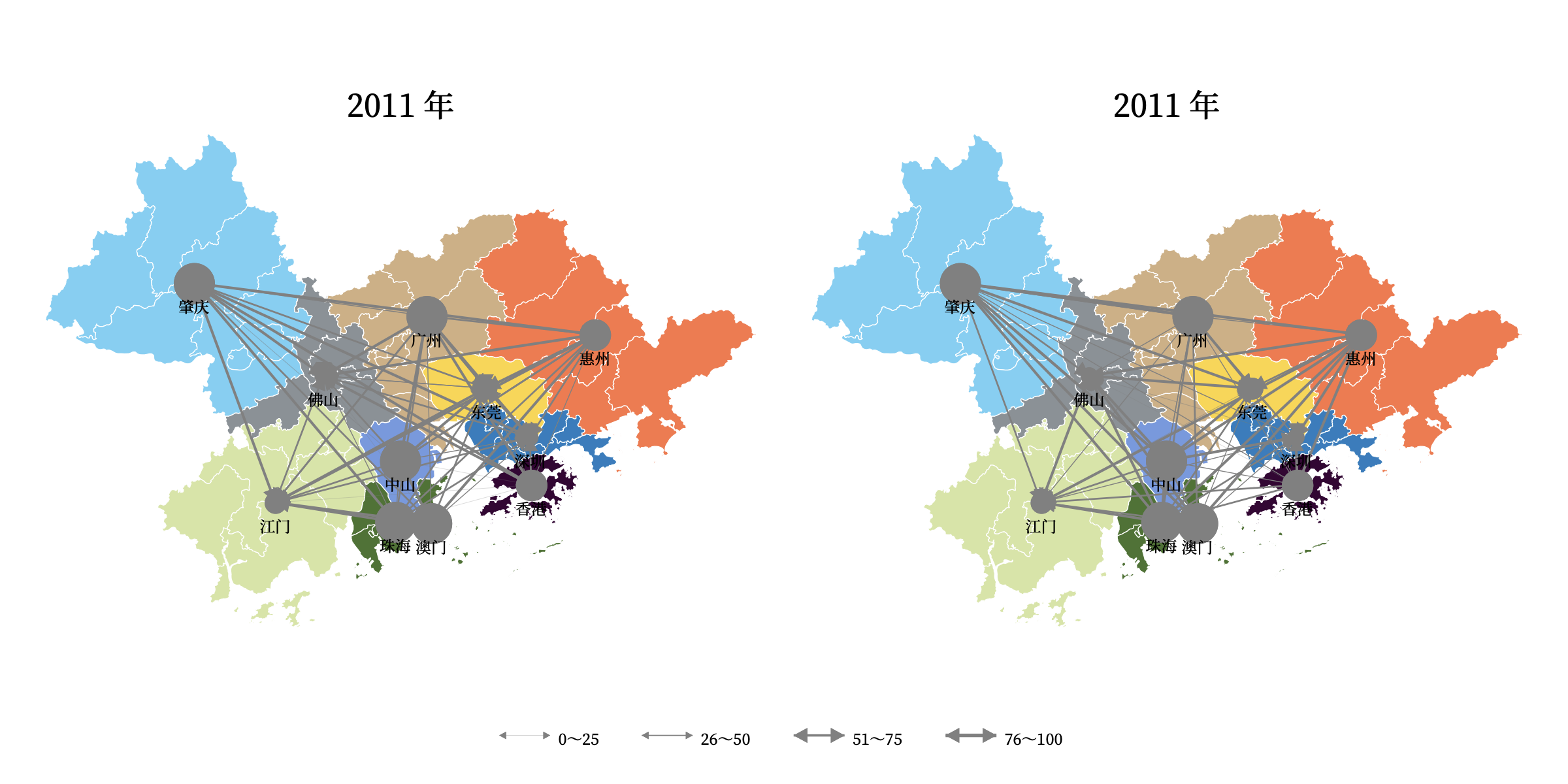
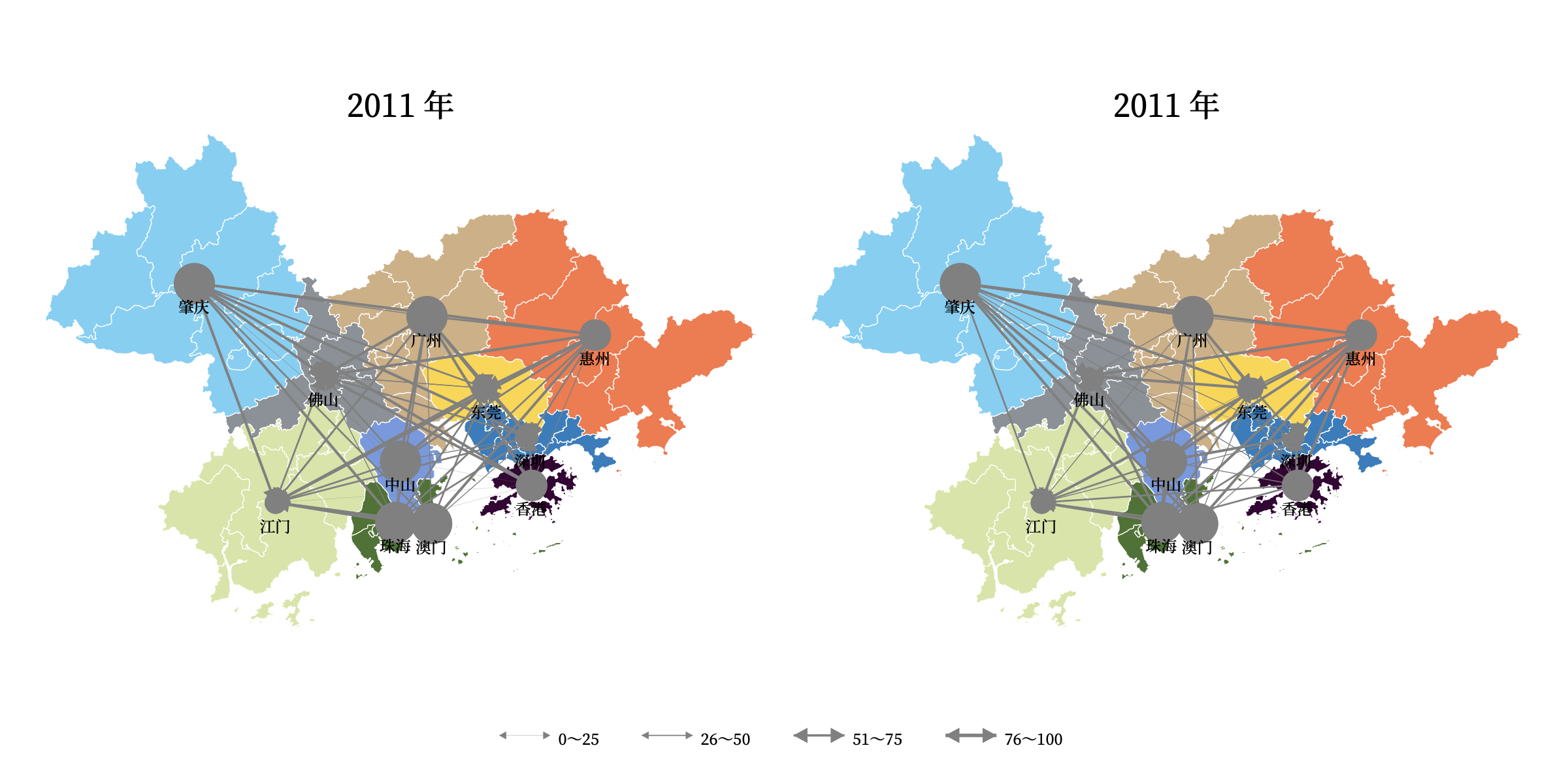
最后我们绘制 2011 和 2020 年数据的对比图,这里使用了 grc1leg 命令合并两幅图并使用相同的图例:
合并多幅地图
use yga_county_db2.dta, clear encode 市, gen (city)tab city if wq, nolabelspmap city using yga_county_coord.dta if wq, id(ID) clmethod(custom) clbreaks(0 1 2 4 5 6 11 13 17 18 19 23) fcolor("254 212 57" "112 154 225" "138 145 151" "210 175 129" "253 116 70" "213 228 162" "25 126 192" "240 92 59" "70 115 46" "113 208 245" "55 3 53" ) ocolor("white" ...) osize(vthin ...) point(data(label ) x(x) y (y) by (group) size(*1 *2 *3 *4) osize(*1.2 ...) shape(O) fcolor(gray ...) ocolor(gray ...)) label (data(label ) x(x) y (y) label (市) gap(*1.8) pos(6) length (6)) graphr(margin(medium)) xsize(9) ysize(6) ti("2011 年" , size(*1.1) pos(12)) arrow(data(arrow) by (group) select(keep if year == 2011) direction(2 ...) legenda(on ) legcount lsize(*0.1 *0.5 *1 *1.5) lcolor(gray ...) hfcolor(gray ...) hocolor(gray ...) hsize(1 1 2 2) hbarbsize(1 1 2 2)) leg(order (17 "0~25" 18 "26~50" 19 "51~75" 20 "76~100" ) symxsize(*2) row(1)) name(a, replace ) spmap city using yga_county_coord.dta if wq, id(ID) clmethod(custom) clbreaks(0 1 2 4 5 6 11 13 17 18 19 23) fcolor("254 212 57" "112 154 225" "138 145 151" "210 175 129" "253 116 70" "213 228 162" "25 126 192" "240 92 59" "70 115 46" "113 208 245" "55 3 53" ) ocolor("white" ...) osize(vthin ...) point(data(label ) x(x) y (y) by (group) size(*1 *2 *3 *4) osize(*1.2 ...) shape(O) fcolor(gray ...) ocolor(gray ...)) label (data(label ) x(x) y (y) label (市) gap(*1.8) pos(6) length (6)) graphr(margin(medium)) xsize(9) ysize(6) ti("2011 年" , size(*1.1) pos(12)) arrow(data(arrow) by (group) select(keep if year == 2020) direction(2 ...) legenda(on ) legcount lsize(*0.1 *0.5 *1 *1.5) lcolor(gray ...) hfcolor(gray ...) hocolor(gray ...) hsize(1 1 2 2) hbarbsize(1 1 2 2)) leg(order (17 "0~25" 18 "26~50" 19 "51~75" 20 "76~100" ) symxsize(*2)) name(b, replace ) grc1leg a b, row(1) legendfrom(a) gr_edit .style.editstyle declared_ysize(5) editcopygr_edit .style.editstyle declared_xsize(10) editcopygr export "粤港澳湾区城市空间网络关系图年份对比.png" , replace width(2400)
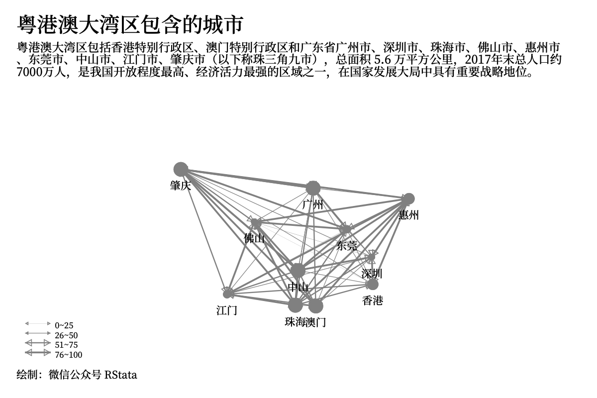
如果想去除地图底图,可以去除填充底图,然后将线条都设置成白色:
无底图
use yga_county_db2.dta, clear encode 市, gen (city)tab city if wq, nolabelspmap using yga_county_coord.dta if wq, id(ID) ocolor(white ...) point(data(label ) x(x) y (y) by (group) size(*0.5 *1 *1.5 *2) osize(*1.2 ...) shape(O) fcolor(gray ...) ocolor(gray ...)) label (data(label ) x(x) y (y) label (市) gap(*1.8) pos(6) length (6)) graphr(margin(medium)) xsize(9) ysize(6) ti("粤港澳大湾区包含的城市" , size(*1.1) pos(11)) subti("粤港澳大湾区包括香港特别行政区、澳门特别行政区和广东省广州市、深圳市、珠海市、佛山市、惠州市" "、东莞市、中山市、江门市、肇庆市(以下称珠三角九市),总面积 5.6 万平方公里,2017年末总人口约" "7000万人,是我国开放程度最高、经济活力最强的区域之一,在国家发展大局中具有重要战略地位。" , size(*0.8) pos(11)) caption("绘制:微信公众号 RStata" , size(*0.8)) arrow(data(arrow) by (group) select(keep if year == 2020) direction(2 ...) legenda(on ) legcount lsize(*0.1 *0.5 *1 *1.5) lcolor(gray ...) hfcolor(gray ...) hocolor(gray ...) hsize(1 1 2 2) hbarbsize(1 1 2 2)) leg(order (7 "0~25" 8 "26~50" 9 "51~75" 10 "76~100" ) symxsize(*2)) gr export "粤港澳湾区城市空间网络关系图2.png" , replace width(1200)
点击这里跳转到 RStata 短书平台获取附件:如何使用 Stata 绘制空间网络图?
评论