使用 Stata 绘图展示 2021 年俄罗斯与各国（地区）间的进出口额

由于俄罗斯对乌克兰的军事行动，西方国家纷纷表示将对俄罗斯实施制裁措施。不过制裁措施是否能发挥效果还得看其与俄罗斯间的进出口关系。

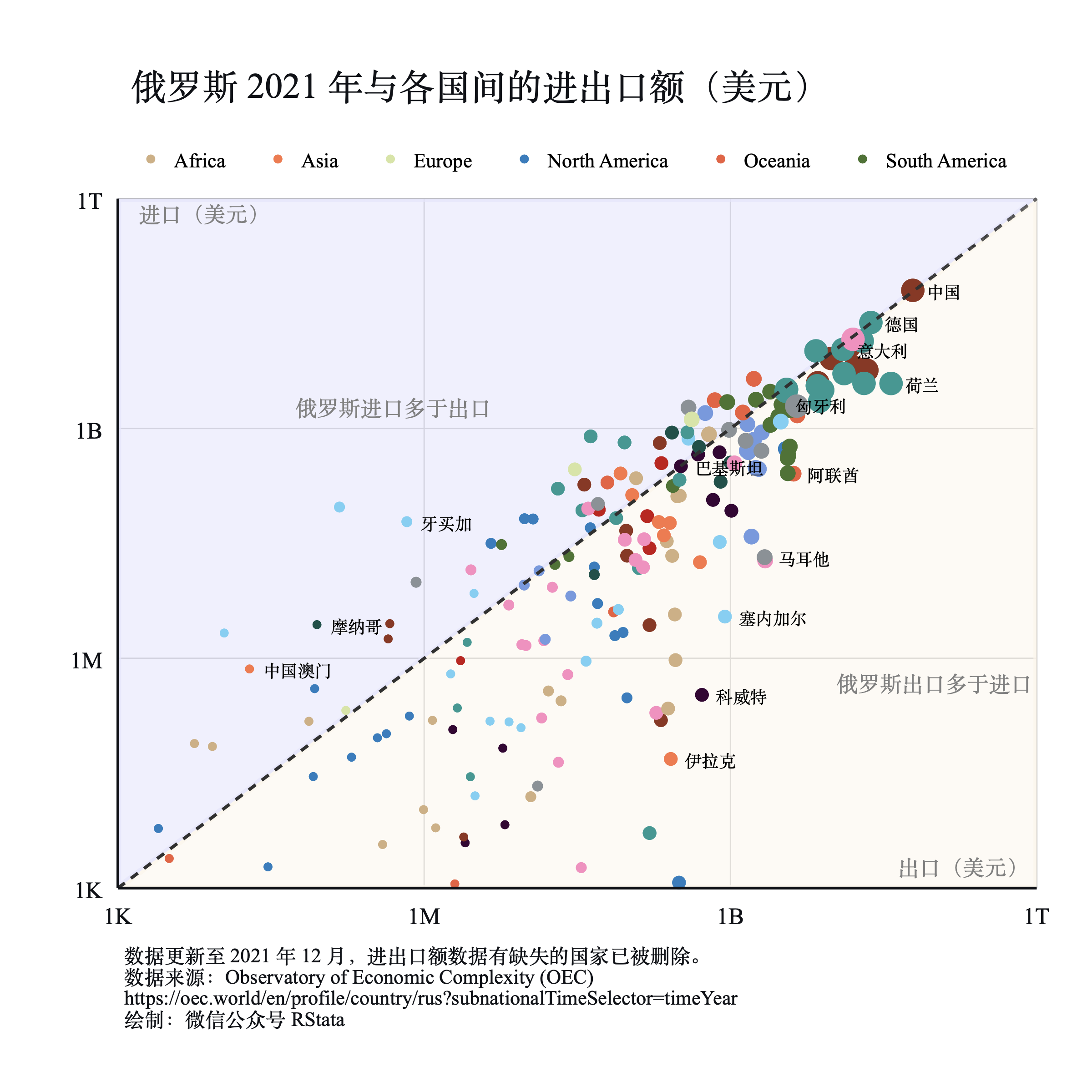
今天我们就用 Stata 来绘制一幅图来展示 2021 年俄罗斯与各个国家（地区）间的进出口额。

图表

首先我们可以从 Observatory of Economic Complexity (OEC) 获取绘图所需的数据，不过还需要整理下（附件中有下面代码所需的数据）：

insheet using "data-iZtV0.csv", clear

由于数据里面的国家名称都是英文的，而我们想绘制一幅中文的地图，我们可以使用数据中的 iso3 变量和 各国ISO对照表.dta 数据匹配得到中文的国家名称：

replace iso3 = strupper(iso3)
merge m:1 iso3 using "各国ISO对照表.dta"
order 国家
drop if _m == 2
gsort _m
drop _m

还有一些没匹配上的手动填补下就可以了：

* 填补下缺失的
replace 国家 = "百慕大" if country == "Bermuda"
replace 国家 = "阿布哈兹" if country == "Abkhazia"
replace 国家 = "摩纳哥" if country == "Monaco"
replace 国家 = "库拉索" if country == "Curaçao"
replace 国家 = "中国澳门" if country == "Macau"
replace 国家 = "南奥塞梯" if country == "South Ossetia"
replace 国家 = "中国台湾" if country == "Taiwan"
replace 国家 = "罗马尼亚" if country == "Romania"
replace 国家 = "塞舍尔" if country == "Seychelles"
replace 国家 = "未知" if country == "Unknown"
replace 国家 = "马绍尔群岛" if country == "Marshall Islands"
replace 国家 = "马尔代夫" if country == "Maldives"
replace 国家 = "巴勒斯坦" if country == "Palestine"
replace 国家 = "中国香港" if country == "Hong Kong"
replace 国家 = "直布罗陀" if country == "Gibraltar"
replace 国家 = "英属维尔京群岛" if country == "British Virgin Islands"
replace 国家 = "圣马力诺" if country == "San Marino"

为了绘制图中的阴影区域，我们需要生成一些辅助变量：

gen x = 1000
replace x = 1000000000000 in `=_N'
gen y = 1000000000000
drop if continent == "NA"

由于 Stata 无法直接把变量值的大小映射给散点的大小，所以我们需要手动生成分组变量，然后对变量进行分组，然后等会儿绘图的时候分多个图层绘制。

* 进出口总额对数
gen sum = log10(import + export)
* 根据进出口总额的对数切分成 10 段：
egen group = cut(sum), group(10)

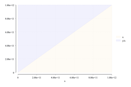
首先绘制图表中的阴影区域：

tw ///
area x x, color("254 247 236%70") || ///
rarea y x x, color("230 230 254%70")

图表

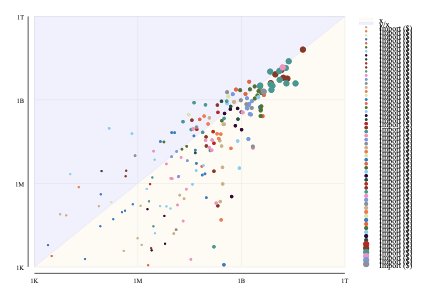
散点图的部分稍微麻烦些，因为我们想给各个大洲的国家使用不同的颜色，又想根据 group 变量给不同的国家使用不同的大小。可以使用循环构造绘图语句：

* 设定绘图主题：
* 安装 ssc install blindschemes, replace
set scheme plotplain, perm
* 绘图
levelsof continent, local(continent)
local cmd = `"tw (area x x, color("254 247 236%70")) (rarea y x x, color("230 230 254%70"))"'
local colorlist = `""75 159 201" "46 95 119" "159 242 209" "184 50 41" "235 145 53" "251 230 165""'
local grouplist = "0.5 0.5 0.7 0.7 1 1 1 1.2 1.2 2"
levelsof group, local(group)
local n = 1
foreach g in `group' {
 local m = 1
 foreach i in `continent' {
  local color: word `m' of `"`colorlist'"'
  local s: word `n' of `grouplist'
  local cmd = `" `cmd' (sc import export if continent == "`i'" & group == `g', m(o) msize(*`s')) "'
  local m = `m' + 1
 }
 local n = `n' + 1
}

`cmd', xsc(log) ///
 ysc(log) ///
 xla(1000 "1K"  ///
  1000000 "1M" ///
  1000000000 "1B" ///
  1000000000000 "1T", noticks ///
  labsize(*0.8) labgap(*2) glp(solid) ///
  glc(gs10) glw(*0.8)) ///
 yla(1000 "1K"  ///
  1000000 "1M" ///
  1000000000 "1B" ///
  1000000000000 "1T", noticks ///
  labsize(*0.8) labgap(*2) glp(solid) ///
  glc(gs10) glw(*0.8)) ///
 xti("") yti("")

图表

上面的部分绘图选项含义如下：

1. xsc(log)：x 轴使用对数轴；
2. ysc(log)：y 轴使用对数轴；
3. xla()、yla()： 设定 x、y 轴的标签；
4. noticks：删除轴线标签上的竖线；
5. labgap()：轴标签与轴的距离（2 倍标准距离）；
6. glp()：grid 的线型；
7. glc()：grid 的颜色；
8. glw()：grid 的粗细。

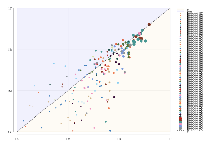
使用 function 可以绘制一条 45 度的斜线：

注意 local 变量的定义和调用要同时运行，所以下面的这段代码还需要和前面 loca cmd = …… 一起选择运行。

`cmd', xsc(log) ///
 ysc(log) ///
 xla(1000 "1K"  ///
  1000000 "1M" ///
  1000000000 "1B" ///
  1000000000000 "1T", noticks ///
  labsize(*0.8) labgap(*2) glp(solid) ///
  glc(gs10) glw(*0.8)) ///
 yla(1000 "1K"  ///
  1000000 "1M" ///
  1000000000 "1B" ///
  1000000000000 "1T", noticks ///
  labsize(*0.8) labgap(*2) glp(solid) ///
  glc(gs10) glw(*0.8)) ///
 xti("") yti("") || ///
function y = x, range(1000 1000000000000) lp(shortdash) ///
 lc(gs3)

图表

lp(shortdash) 表示斜线使用小短线；lc(gs3) 表示斜线使用 30 度灰。

下面我们再把图例修修：

`cmd', xsc(log) ///
 ysc(log) ///
 xla(1000 "1K"  ///
  1000000 "1M" ///
  1000000000 "1B" ///
  1000000000000 "1T", noticks ///
  labsize(*0.8) labgap(*2) glp(solid) ///
  glc(gs10) glw(*0.8)) ///
 yla(1000 "1K"  ///
  1000000 "1M" ///
  1000000000 "1B" ///
  1000000000000 "1T", noticks ///
  labsize(*0.8) labgap(*2) glp(solid) ///
  glc(gs10) glw(*0.8)) ///
 xti("") yti("") || ///
function y = x, range(1000 1000000000000) lp(shortdash) ///
 lc(gs3) ///
 plotr(margin(zero)) ///
 text(680000000000 7000 "进口（美元）", size(*0.6) color(gray)) ///
 text(2000 190000000000 "出口（美元）", size(*0.6) color(gray)) ///
 ti("俄罗斯 2021 年与各国间的进出口额（美元）", size(*0.7)) ///
 caption("数据更新至 2021 年 12 月，进出口额数据有缺失的国家已被删除。" ///
  "数据来源：Observatory of Economic Complexity (OEC)" ///
  "https://oec.world/en/profile/country/rus?subnationalTimeSelector=timeYear" ///
  "绘制：微信公众号 RStata", ///
  pos(5) size(*0.7) justification(left) bexpand) ///
 graphr(margin(medlarge)) ///
 leg(order(3 "Africa" 4 "Asia" 5 "Europe" ///
  6 "North America" 7 "Oceania" ///
  8 "South America") pos(11) row(1) ///
  size(*0.7)) ///
 ysize(20) xsize(20)

这里的两个 text() 选项是为了添加横纵轴的标题；plotr(margin(zero)) 表示 plot 区域的边距为 0；leg(order()) 是设置图例的，这里选择 3-8 号图层进行标注（每个图层对应什么可以从绘图代码里面数）：

di `"`cmd'"'

*> tw (area x x, color
*> > ("254 247 236%70")) (rarea y x x, color("230 230 254%70")) (sc import export
*> > if continent == "Africa" & group == 0, m(o) msize(*0.5))  (sc import export i
*> > f continent == "Asia" & group == 0, m(o) msize(*0.5))  (sc import export if c
*> > ontinent == "Europe" & group == 0, m(o) msize(*0.5))  (sc import export if co
*> > ntinent == "North America" & group == 0, m(o) msize(*0.5))  (sc import export
*> >  if continent == "Oceania" & group == 0, m(o) msize(*0.5))  (sc import export
*> >  if continent == "South America" & group == 0, m(o) msize(*0.5))  (sc import
*> > export if continent == "Africa" & group == 1, m(o) msize(*0.5))  (sc import e
*> > xport if continent == "Asia" & group == 1, m(o) msize(*0.5))  (sc import expo
*> > rt if continent == "Europe" & group == 1, m(o) msize(*0.5))  (sc import expor
*> > t if continent == "North America" & group == 1, m(o) msize(*0.5))  (sc import
*> >  export if continent == "Oceania" & group == 1, m(o) msize(*0.5))  (sc import
*> >  export if continent == "South America" & group == 1, m(o) msize(*0.5))  (sc
*> > import export if continent == "Africa" & group == 2, m(o) msize(*0.7))  (sc i
*> > mport export if continent == "Asia" & group == 2, m(o) msize(*0.7))  (sc impo
*> > rt export if continent == "Europe" & group == 2, m(o) msize(*0.7))  (sc impor
*> > t export if continent == "North America" & group == 2, m(o) msize(*0.7))  (sc
*> >  import export if continent == "Oceania" & group == 2, m(o) msize(*0.7))  (sc
*> >  import export if continent == "South America" & group == 2, m(o) msize(*0.7)
*> > )  (sc import export if continent == "Africa" & group == 3, m(o) msize(*0.7))
*> >   (sc import export if continent == "Asia" & group == 3, m(o) msize(*0.7))  (
*> > sc import export if continent == "Europe" & group == 3, m(o) msize(*0.7))  (s
*> > c import export if continent == "North America" & group == 3, m(o) msize(*0.7
*> > ))  (sc import export if continent == "Oceania" & group == 3, m(o) msize(*0.7
*> > ))  (sc import export if continent == "South America" & group == 3, m(o) msiz
*> > e(*0.7))  (sc import export if continent == "Africa" & group == 4, m(o) msize
*> > (*1))  (sc import export if continent == "Asia" & group == 4, m(o) msize(*1))
*> >   (sc import export if continent == "Europe" & group == 4, m(o) msize(*1))  (
*> > sc import export if continent == "North America" & group == 4, m(o) msize(*1)
*> > )  (sc import export if continent == "Oceania" & group == 4, m(o) msize(*1))
*> >  (sc import export if continent == "South America" & group == 4, m(o) msize(*
*> > 1))  (sc import export if continent == "Africa" & group == 5, m(o) msize(*1))
*> >   (sc import export if continent == "Asia" & group == 5, m(o) msize(*1))  (sc
*> >  import export if continent == "Europe" & group == 5, m(o) msize(*1))  (sc im
*> > port export if continent == "North America" & group == 5, m(o) msize(*1))  (s
*> > c import export if continent == "Oceania" & group == 5, m(o) msize(*1))  (sc
*> > import export if continent == "South America" & group == 5, m(o) msize(*1))
*> > (sc import export if continent == "Africa" & group == 6, m(o) msize(*1))  (sc
*> >  import export if continent == "Asia" & group == 6, m(o) msize(*1))  (sc impo
*> > rt export if continent == "Europe" & group == 6, m(o) msize(*1))  (sc import
*> > export if continent == "North America" & group == 6, m(o) msize(*1))  (sc imp
*> > ort export if continent == "Oceania" & group == 6, m(o) msize(*1))  (sc impor
*> > t export if continent == "South America" & group == 6, m(o) msize(*1))  (sc i
*> > mport export if continent == "Africa" & group == 7, m(o) msize(*1.2))  (sc im
*> > port export if continent == "Asia" & group == 7, m(o) msize(*1.2))  (sc impor
*> > t export if continent == "Europe" & group == 7, m(o) msize(*1.2))  (sc import
*> >  export if continent == "North America" & group == 7, m(o) msize(*1.2))  (sc
*> > import export if continent == "Oceania" & group == 7, m(o) msize(*1.2))  (sc
*> > import export if continent == "South America" & group == 7, m(o) msize(*1.2))
*> >   (sc import export if continent == "Africa" & group == 8, m(o) msize(*1.2))
*> >  (sc import export if continent == "Asia" & group == 8, m(o) msize(*1.2))  (s
*> > c import export if continent == "Europe" & group == 8, m(o) msize(*1.2))  (sc
*> >  import export if continent == "North America" & group == 8, m(o) msize(*1.2)
*> > )  (sc import export if continent == "Oceania" & group == 8, m(o) msize(*1.2)
*> > )  (sc import export if continent == "South America" & group == 8, m(o) msize
*> > (*1.2))  (sc import export if continent == "Africa" & group == 9, m(o) msize(
*> > *2))  (sc import export if continent == "Asia" & group == 9, m(o) msize(*2))
*> >  (sc import export if continent == "Europe" & group == 9, m(o) msize(*2))  (s
*> > c import export if continent == "North America" & group == 9, m(o) msize(*2))
*> >   (sc import export if continent == "Oceania" & group == 9, m(o) msize(*2))
*> > (sc import export if continent == "South America" & group == 9, m(o) msize(*2
*> > )) *>

可以看到 area 和 rarea 图层是第一、二号图层，然后 3——8 正好是几个大洲的散点图层。后面的再数起来就比较困难了。

我们再使用一个散点图层添加一些散点标签：

`cmd', xsc(log) ///
 ysc(log) ///
 xla(1000 "1K"  ///
  1000000 "1M" ///
  1000000000 "1B" ///
  1000000000000 "1T", noticks ///
  labsize(*0.8) labgap(*2) glp(solid) ///
  glc(gs10) glw(*0.8)) ///
 yla(1000 "1K"  ///
  1000000 "1M" ///
  1000000000 "1B" ///
  1000000000000 "1T", noticks ///
  labsize(*0.8) labgap(*2) glp(solid) ///
  glc(gs10) glw(*0.8)) ///
 xti("") yti("") || ///
function y = x, range(1000 1000000000000) lp(shortdash) ///
 lc(gs3) ///
 plotr(margin(zero)) ///
 text(680000000000 7000 "进口（美元）", size(*0.6) color(gray)) ///
 text(2000 190000000000 "出口（美元）", size(*0.6) color(gray)) ///
 ti("俄罗斯 2021 年与各国间的进出口额（美元）", size(*0.7)) ///
 caption("数据更新至 2021 年 12 月，进出口额数据有缺失的国家已被删除。" ///
  "数据来源：Observatory of Economic Complexity (OEC)" ///
  "https://oec.world/en/profile/country/rus?subnationalTimeSelector=timeYear" ///
  "绘制：微信公众号 RStata", ///
  pos(5) size(*0.7) justification(left) bexpand) ///
 graphr(margin(medlarge)) ///
 leg(order(3 "Africa" 4 "Asia" 5 "Europe" ///
  6 "North America" 7 "Oceania" ///
  8 "South America") pos(11) row(1) ///
  size(*0.7)) ///
 ysize(20) xsize(20) || ///
 sc import export if ///
  inlist(country, "China", "Germany", ///
   "Netherlands", "Italy", "Hungary", ///
   "United Arab Emirates", "Pakistan", ///
   "Malta", "Senegal") | ///
  inlist(country, "Iraq", "Kuwait", ///
   "Macau", "Monaco", "Jamaica"), ///
  m(i) mlab(国家) mlabsize(*0.6) mlabcolor(black) ///
  text(2000000000 500000 "俄罗斯进口多于出口", size(*0.6) color(gray)) ///
  text(500000 100000000000 "俄罗斯出口多于进口", size(*0.6) color(gray))

这里的 m(i) 就表示隐藏散点，仅仅显示标签。由于 inlist() 函数仅仅支持 <= 9 个条件，所以我使用了 inlsit() | inlist()。

最后，这幅图的完整代码是：

insheet using "data-iZtV0.csv", clear
replace iso3 = strupper(iso3)
merge m:1 iso3 using "各国ISO对照表.dta"
order 国家
drop if _m == 2
gsort _m
drop _m
* 填补下缺失的
replace 国家 = "百慕大" if country == "Bermuda"
replace 国家 = "阿布哈兹" if country == "Abkhazia"
replace 国家 = "摩纳哥" if country == "Monaco"
replace 国家 = "库拉索" if country == "Curaçao"
replace 国家 = "中国澳门" if country == "Macau"
replace 国家 = "南奥塞梯" if country == "South Ossetia"
replace 国家 = "中国台湾" if country == "Taiwan"
replace 国家 = "罗马尼亚" if country == "Romania"
replace 国家 = "塞舍尔" if country == "Seychelles"
replace 国家 = "未知" if country == "Unknown"
replace 国家 = "马绍尔群岛" if country == "Marshall Islands"
replace 国家 = "马尔代夫" if country == "Maldives"
replace 国家 = "巴勒斯坦" if country == "Palestine"
replace 国家 = "中国香港" if country == "Hong Kong"
replace 国家 = "直布罗陀" if country == "Gibraltar"
replace 国家 = "英属维尔京群岛" if country == "British Virgin Islands"
replace 国家 = "圣马力诺" if country == "San Marino"

* 生成辅助变量
gen x = 1000
replace x = 1000000000000 in `=_N'
gen y = 1000000000000
drop if continent == "NA"

* 进出口总额对数
gen sum = log10(import + export)
* 根据进出口总额的对数切分成 10 段：
egen group = cut(sum), group(10)

* 绘图
levelsof continent, local(continent)
local cmd = `"tw (area x x, color("254 247 236%70")) (rarea y x x, color("230 230 254%70"))"'
local colorlist = `""75 159 201" "46 95 119" "159 242 209" "184 50 41" "235 145 53" "251 230 165""'
local grouplist = "0.5 0.5 0.7 0.7 1 1 1 1.2 1.2 2"
levelsof group, local(group)
local n = 1
foreach g in `group' {
 local m = 1
 foreach i in `continent' {
  local color: word `m' of `"`colorlist'"'
  local s: word `n' of `grouplist'
  local cmd = `" `cmd' (sc import export if continent == "`i'" & group == `g', m(o) msize(*`s')) "'
  local m = `m' + 1
 }
 local n = `n' + 1
}

`cmd', xsc(log) ///
 ysc(log) ///
 xla(1000 "1K"  ///
  1000000 "1M" ///
  1000000000 "1B" ///
  1000000000000 "1T", noticks ///
  labsize(*0.8) labgap(*2) glp(solid) ///
  glc(gs10) glw(*0.8)) ///
 yla(1000 "1K"  ///
  1000000 "1M" ///
  1000000000 "1B" ///
  1000000000000 "1T", noticks ///
  labsize(*0.8) labgap(*2) glp(solid) ///
  glc(gs10) glw(*0.8)) ///
 xti("") yti("") || ///
function y = x, range(1000 1000000000000) lp(shortdash) ///
 lc(gs3) ///
 plotr(margin(zero)) ///
 text(680000000000 7000 "进口（美元）", size(*0.6) color(gray)) ///
 text(2000 190000000000 "出口（美元）", size(*0.6) color(gray)) ///
 ti("俄罗斯 2021 年与各国间的进出口额（美元）", size(*0.7)) ///
 caption("数据更新至 2021 年 12 月，进出口额数据有缺失的国家已被删除。" ///
  "数据来源：Observatory of Economic Complexity (OEC)" ///
  "https://oec.world/en/profile/country/rus?subnationalTimeSelector=timeYear" ///
  "绘制：微信公众号 RStata", ///
  pos(5) size(*0.7) justification(left) bexpand) ///
 graphr(margin(medlarge)) ///
 leg(order(3 "Africa" 4 "Asia" 5 "Europe" ///
  6 "North America" 7 "Oceania" ///
  8 "South America") pos(11) row(1) ///
  size(*0.7)) ///
 ysize(20) xsize(20) || ///
 sc import export if ///
  inlist(country, "China", "Germany", ///
   "Netherlands", "Italy", "Hungary", ///
   "United Arab Emirates", "Pakistan", ///
   "Malta", "Senegal") | ///
  inlist(country, "Iraq", "Kuwait", ///
   "Macau", "Monaco", "Jamaica"), ///
  m(i) mlab(国家) mlabsize(*0.6) mlabcolor(black) ///
  text(2000000000 500000 "俄罗斯进口多于出口", size(*0.6) color(gray)) ///
  text(500000 100000000000 "俄罗斯出口多于进口", size(*0.6) color(gray))

gr export "俄罗斯 2021 年与各国间的进出口额（美元）.png", replace width(2400)
gr export "俄罗斯 2021 年与各国间的进出口额（美元）.pdf", replace

图表

点击这里跳转到 RStata 短书平台获取附件：使用 Stata 绘图展示 2021 年俄罗斯与各国（地区）间的进出口额